[home]   [coding projects]   [research projects]   [research interests]

Scalable Interpolation

A manual for the MapReduce interpolation implementations and finite-recurrence reconstruction experiments.

This project is both an implementation library and an experiment harness for interpolation under MapReduce. Classical methods are implemented alongside a custom finite-recurrence reconstruction method, then the methods are pushed through the same size, accuracy, and extrapolation tests.

The useful way to read the code is not as “twelve interpolation functions.” The central idea is that sampled values can be compressed into a short recurrence, and that the recurrence can be continued in either direction without reconstructing one enormous global polynomial.

Contents

1. Pipeline

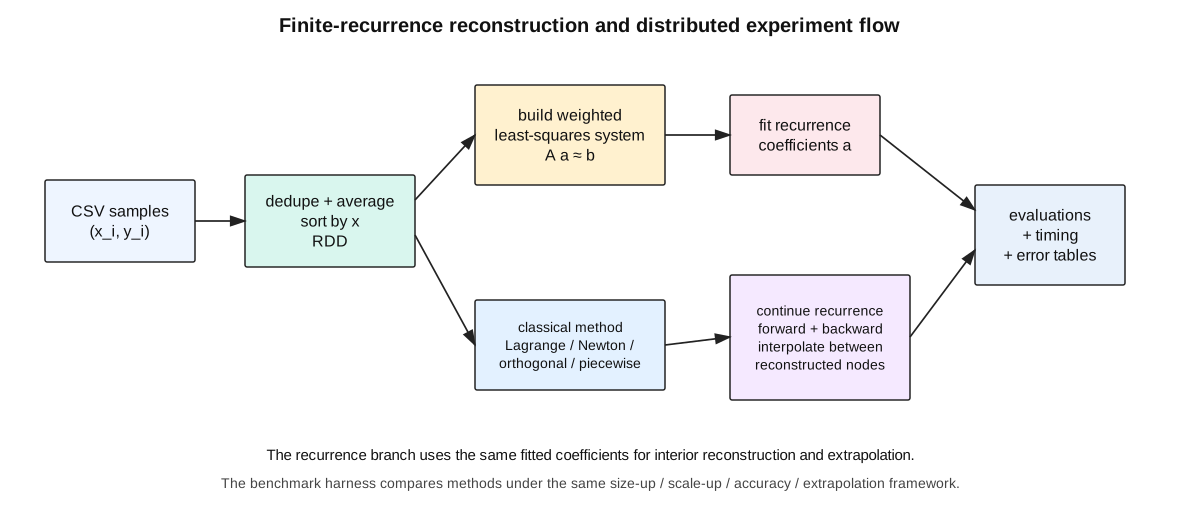
Input CSV rows are converted to an RDD of \((x,y)\) pairs. Duplicate \(x\)-values are reduced by averaging their \(y\)-values, the nodes are sorted, and the same cleaned sample set can then be passed to any interpolation engine.

The source includes direct Lagrange, first- and second-form barycentric Lagrange, Newton divided differences, Neville, Aitken, Chebyshev, Legendre, Jacobi, piecewise Lagrange, and piecewise Newton implementations. For large profiles the experiment narrows to the methods that remain practical at that scale.

2. Fitting the finite recurrence

For an order-\(k\) model, the sampled values are treated as approximately satisfying

The implementation forms one weighted least-squares row per usable sample position and solves for the coefficient vector \(a\):

def fit_recurrence(y, X_vals, k):
    m = len(y) - k
    A_rows = []
    b_vals = []

    for i in range(m):
        xi = X_vals[i + k]
        xikm1 = X_vals[i + k - 1]
        xim1 = X_vals[i - 1] if i - 1 >= 0 else X_vals[0]

        denom = xi - xim1
        if abs(denom) < eps:
            weight = 1.0
        else:
            weight = (xi - xikm1) / denom

        A_rows.append(weight * y[i:i+k])
        b_vals.append(weight * y[i+k])

    A = np.vstack(A_rows)
    b = np.array(b_vals)

    coef, _, _, _ = np.linalg.lstsq(A, b, rcond=None)
    return coef

The important computational feature is that the recurrence order is fixed while the number of samples can be large. The fit therefore reduces a long sampled sequence to a small coefficient vector rather than retaining a separate polynomial coefficient for every interpolation node.

3. Forward and backward continuation

The recurrence is fitted twice: once to the data in forward order and once to the reversed data. The forward fit is used to continue beyond the right boundary; the reversed fit supplies the corresponding continuation beyond the left boundary.

a_fwd = fit_recurrence(Y, X, k)

Y_rev = Y[::-1]
X_rev = X[::-1]
a_bwd = fit_recurrence(Y_rev, X_rev, k)

F = np.zeros(max_right_idx, dtype=float)
F[:n] = Y
for i in range(n, max_right_idx):
    F[i] = np.dot(a_fwd, F[i-k:i])

B = np.zeros(max_left_j, dtype=float)
B[:n] = Y_rev
for j in range(n, max_left_j):
    B[j] = np.dot(a_bwd, B[j-k:j])

A later version of the function also builds recurrence-generated values across the interior from both directions and blends the forward and backward predictions, while keeping the endpoints exact. Evaluation between reconstructed nodes is then piecewise linear on the actual \(X\)-grid.

4. Classical baselines

The classical methods are not filler: they make the recurrence method interpretable. The code contains both global and local baselines, direct and barycentric Lagrange forms, divided-difference and table recursions, and orthogonal-polynomial bases. The same evaluation functions can therefore ask whether a method scales, whether it is accurate on a given node distribution, and whether it behaves sensibly outside the sampled interval.

5. Benchmark profiles

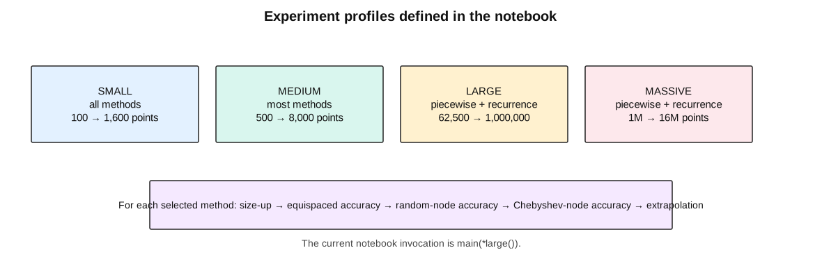
The benchmark code has separate routines for speed-up, size-up, scale-up, equispaced accuracy, random-node accuracy, Chebyshev-node accuracy, and extrapolation. The main routine applies the same battery to each selected interpolation function.

print("--------------- SIZEUP BEGIN ---------------")
df_sizeup = run_sizeup_experiments(...)

print("--------------- EQUISPACED BEGIN ---------------")
df_eq = run_accuracy_equispaced(spark, fn, acc_ns)

print("--------------- RANDOM BEGIN ---------------")
df_rand = run_accuracy_random(spark, fn, acc_ns, seed=0)

print("--------------- CHEBYSHEV BEGIN ---------------")
df_cheb = run_accuracy_chebyshev(spark, fn, acc_ns)

print("--------------- EXTRAPOLATION BEGIN ---------------")
df_ex = run_extrapolation_experiments(
    spark=spark,
    interpolation_fn=fn,
    acc_ns=acc_ns,
    shifts=shifts
)

6. Running the notebook

This source was written as a Colab/PySpark experiment. It creates a local Spark session, mounts Google Drive, and expects the profile data beneath the configured Drive paths. At the bottom of the current source, the large profile is active:

# main(*massive())
main(*large())
# main(*medium())
# main(*small())

The profile functions determine both the set of algorithms and the scale of the data. For example, the large profile uses the two piecewise methods plus the quotient-ring recurrence method at sizes from 62,500 to 1,000,000 nodes, while the small profile includes all of the classical methods.

Related research

Scalable Interpolation under MapReduce via Finite-Recurrence Reconstruction

These pages are selective technical manuals: enough source to expose the mechanism, not a mirror of the entire repository.
Last updated: September 14, 2026.